Variants of Gradient Boosting
How to reduce this Time complexity in this algorithm when we are using Big datasets

Approach 2 -Histogram Based Algorithms
IDEA 1
Use the Histograms to find the Bins for each feature
Use this bins to find the best split (This is supported by the fact that the Spliting on real value or bins does't cost much difference in accuracy)
Note : USing bins may also prevents from Overfiting

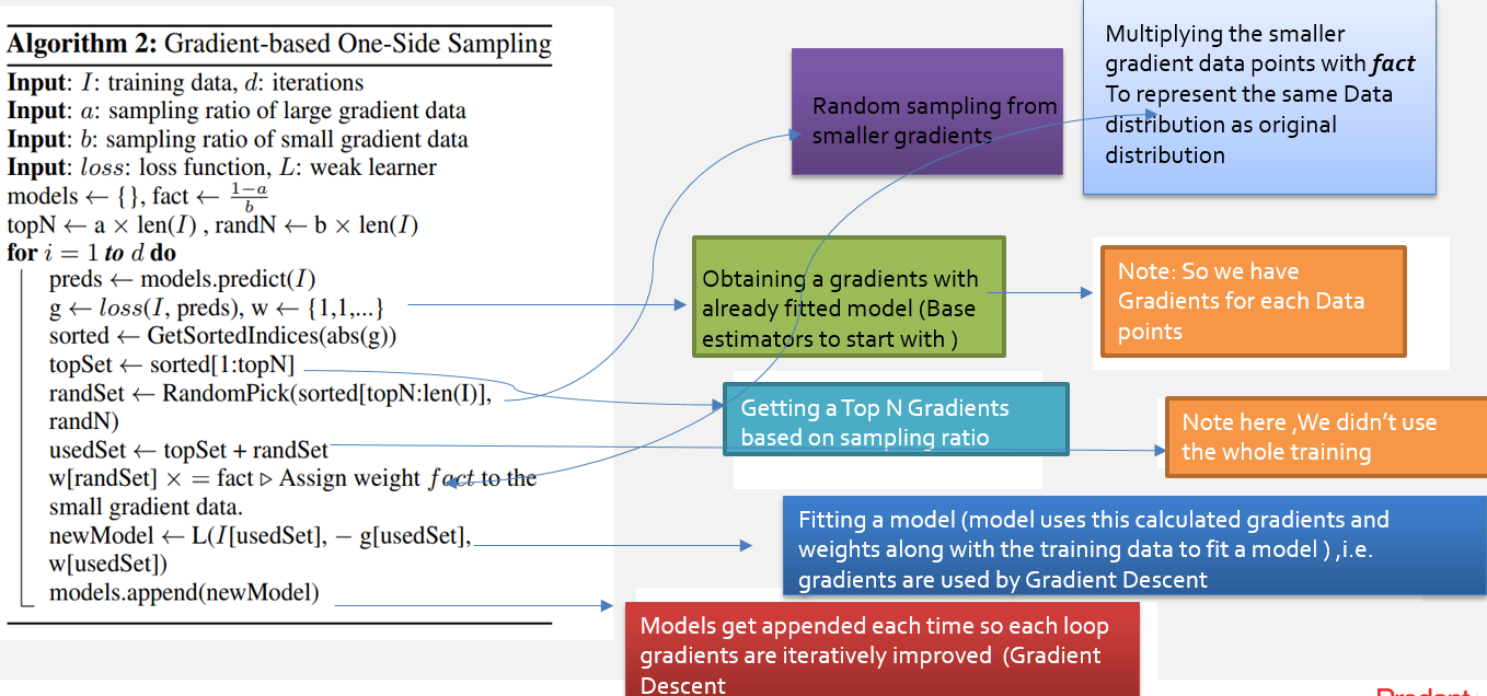
Taking Sparsity of the data as advantage
Ignoring sparse inputs (xgboost and lightGBM)
Xgboost proposes to ignore the 0 features when computing the split, then allocating all the data with missing values to whichever side of the split reduces the loss more. This reduces the number of samples that have to be used when evaluating each split, speeding up the training process.

In [3]:
from sklearn.ensemble import GradientBoostingClassifier,GradientBoostingRegressor
from sklearn.datasets import load_boston,load_wine
import pandas as pd
from sklearn.model_selection import train_test_split
import matplotlib.pyplot as plt
from sklearn import metrics
import math
import numpy as np

def rmse(x,y): return math.sqrt(((x-y)**2).mean())

def print_score(m):
    res = [rmse(m.predict(X_train), y_train), rmse(m.predict(X_test), y_test),
                m.score(X_train, y_train), m.score(X_test, y_test)]
    if hasattr(m, 'oob_score_'): res.append(m.oob_score_)
    print(res)
house_price=load_boston(return_X_y=False)
#house_price['data']
#house_price['feature_names']
#house_price['target']
X_df=pd.DataFrame(data=house_price['data'],columns=house_price['feature_names'])
y=house_price['target']
X_df.head(10)
Out[3]:
In [12]:
X_df.nunique()
Out[12]:
Catboost DEMO
In [45]:
#pred=m.predict(X_test)
plt.plot(y_test,label='orig')
plt.plot(preds1,label='pred')
plt.legend()
plt.show()
rmse(y_test,preds1)

Out[45]:
In [28]:
#pred=m.predict(X_test)
plt.plot(y_test,label='orig')
plt.plot(preds,label='pred')
plt.legend()
plt.show()
rmse(y_test,preds)

Out[28]:
Reference :
- https://blogs.technet.microsoft.com/machinelearning/2017/07/25/lessons-learned-benchmarking-fast-machine-learning-algorithms/
- http://mlexplained.com/2018/01/05/lightgbm-and-xgboost-explained/
- https://github.com/Microsoft/LightGBM/blob/master/docs/Features.rst
- https://towardsdatascience.com/catboost-vs-light-gbm-vs-xgboost-5f93620723db