Tree vs Forest
Lets See the Practical problems in Decision Tree -
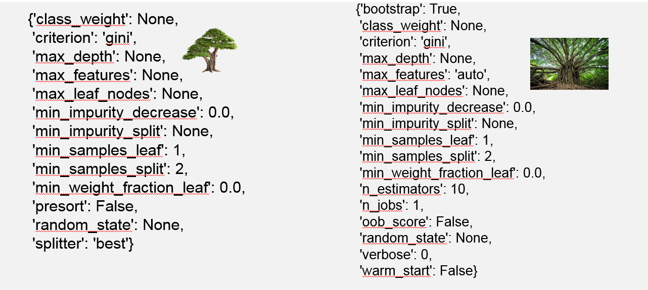
Lets have a look at Decision Tree's Hyperparameters
from sklearn.tree import DecisionTreeClassifier,DecisionTreeRegressor
from sklearn.ensemble import RandomForestClassifier,RandomForestRegressor
Decision tree Paramaters and Attributes
dtr=DecisionTreeClassifier()
dtr.get_params
DecisionTreeClassifier??
dir(dtr)
Drawbacks of Descision Tree Based Modeling
- Prune to Overfiting !!
- They are unstable, meaning that a small change in the data can lead to a large change in the structure of the optimal decision tree.
- They are often relatively inaccurate. Many other predictors perform better with similar data. This can be remedied by replacing a single decision tree with a random forest of decision trees, but a random forest is not as easy to interpret as a single decision tree.
- For data including categorical variables with different number of levels, information gain in decision trees is biased in favor of those attributes with more levels
- Calculations can get very complex, particularly if many values are uncertain and/or if many outcomes are linked
What is a Good Decision ??
- Single Individual's decision won't be a good decision all the time (sometimes though)
- Good Decision and Bad Decision are again subjective  (varies from person to person ,situation to situation)
- ## Atlast everything is all about statisfaction
Why Random Forest works well/better in practice !?
Physcological perspective :
- Find the solution for the particular problem based on knowledge /suggestion from many such individuals and decide accordingly
- Choose those individuals wisely
There was another Experiement Related to the Neuroscience
(easy to explain hard to write)Random Forest
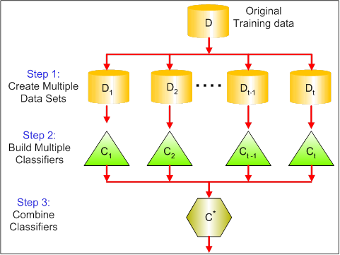
Ensemble (together):
Ensemble  is a collection of learners (base estimators ) which in turn builts the Strong Predictor or Learning strategy

You can combine any predictor or learning algorithms (not just trees) to achieve your end goal (high accuarcy )
(but consider Generilization Error)
Types of Ensemble modeling
- Bagging
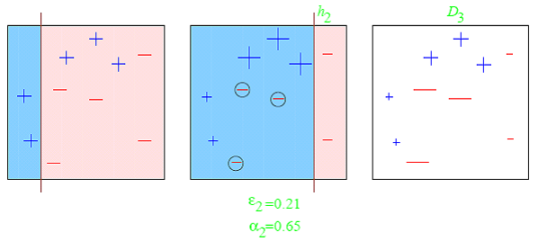
- Boosting
- Stacking
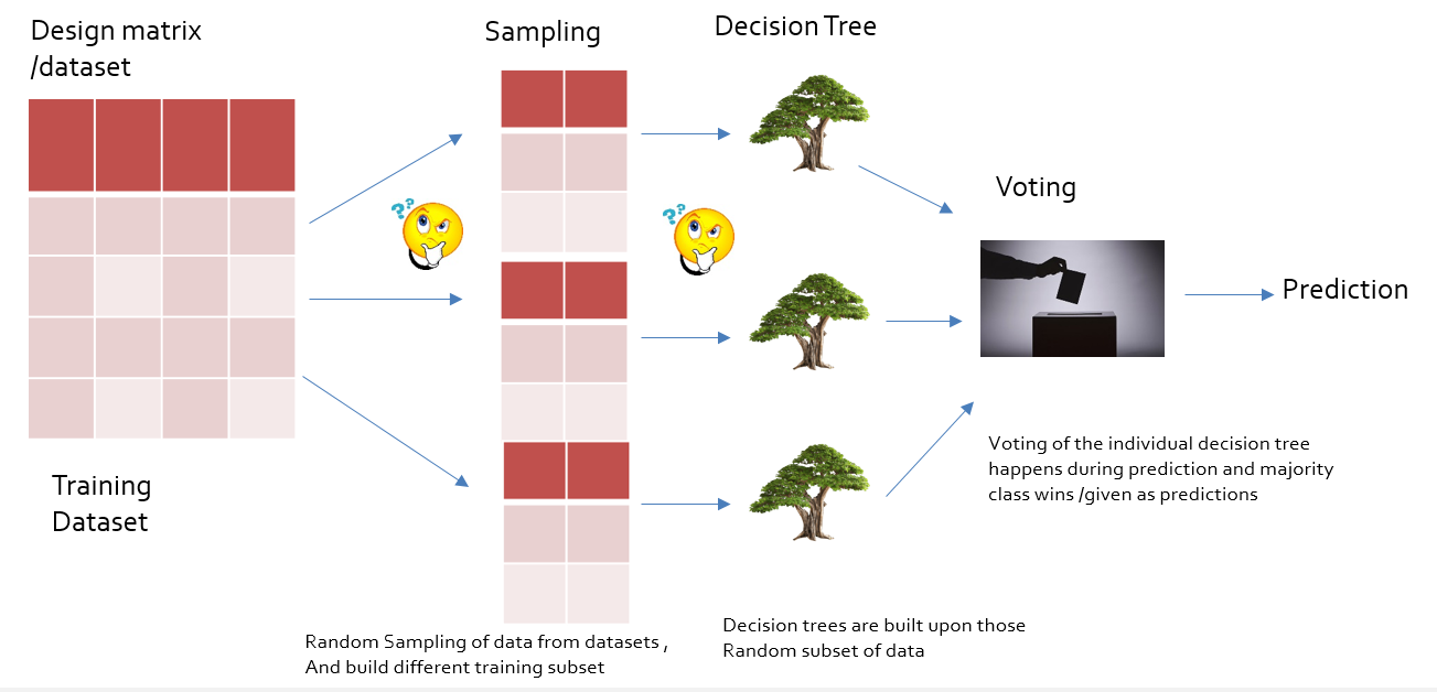
Bagging (Random Forest )
Boosting (Gradient Boosting)
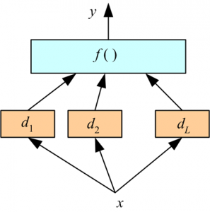
Stacking (stacking two or three models)
Success of Ensemble Modeling
Success of your model really lies in modeling each individual tree as different as possible (uncorrelated )
How to achieve the possible differnce between the models ?
- Difference in population
- Difference in hypothesis
- Difference in modeling technique
- Difference in initial seed
Refrence :
Hyperparameters for Decision Tree and Random Forest
TIPS and Tricks to Use RandomForest for various things
from sklearn.datasets import load_boston,load_wine
import pandas as pd
from sklearn.model_selection import train_test_split
import matplotlib.pyplot as plt
from sklearn import metrics
import math
import numpy as np
from sklearn.ensemble import RandomForestClassifier,RandomForestRegressor
def rmse(x,y): return math.sqrt(((x-y)**2).mean())

def print_score(m):
    res = [rmse(m.predict(X_train), y_train), rmse(m.predict(X_test), y_test),
                m.score(X_train, y_train), m.score(X_test, y_test)]
    if hasattr(m, 'oob_score_'): res.append(m.oob_score_)
    print(res)
house_price=load_boston(return_X_y=False)
#house_price['data']
#house_price['feature_names']
#house_price['target']
X_df=pd.DataFrame(data=house_price['data'],columns=house_price['feature_names'])
y=house_price['target']
X_df.head(10)
plt.plot(y)
plt.show()

m.estimators_
preds = np.stack([t.predict(X_test) for t in m.estimators_])
preds[:,0], np.mean(preds[:,0]), y_test[0]
preds.shape
pred=m.predict(X_test)
interval=+np.std(preds)
index=list(range(len(pred)))
Getting Confidence interval
plt.figure()
plt.plot(index,pred)

#plt.plot(dataframe.index,dataframe[col_name],label='original')
#plt.plot(dataframe.index,predicted_gb,label='predicted gradient descent')
#plt.plot(dataframe.index,upper,label='upper_boundary')
#plt.plot(dataframe.index,lower,label='lower_boundary')
lower=pred-np.std(preds)
upper=pred+np.std(preds)
plt.xticks(rotation=80)
plt.xlabel('index')
plt.ylabel('pred')
plt.fill_between(index,lower,upper,alpha=0.4)
plt.show()

plt.plot(pred+np.std(preds))
plt.show()

list(zip(house_price['feature_names'],m.feature_importances_))
plt.plot([metrics.r2_score(y_test, np.mean(preds[:i+1], axis=0)) for i in range(10)])
plt.xlabel('No of estimators')
plt.ylabel('r2 score')
plt.show()

m = RandomForestRegressor(n_estimators=20, n_jobs=-1)
m.fit(X_train, y_train)
print_score(m)
m = RandomForestRegressor(n_estimators=40, n_jobs=-1)
m.fit(X_train, y_train)
print_score(m)
m = RandomForestRegressor(n_estimators=80, n_jobs=-1)
m.fit(X_train, y_train)
print_score(m)
Hierarchical Clustering
import scipy
from scipy.cluster import hierarchy as hc
corr = np.round(scipy.stats.spearmanr(X_df).correlation, 4)
corr_condensed = hc.distance.squareform(1-corr)
z = hc.linkage(corr_condensed, method='average')
fig = plt.figure(figsize=(16,10))
dendrogram = hc.dendrogram(z, labels=X_df.columns, orientation='left', leaf_font_size=16)
plt.show()

!pip install pdpbox
rf=RandomForestRegressor()
from sklearn.linear_model import LinearRegression
rf.base_estimator=LinearRegression
rf.n_estimators
pdpbox
When using black box machine learning algorithms like random forest and boosting, it is hard to understand the relations between predictors and model outcome.
For example, in terms of random forest, all we get is the feature importance. Although we can know which feature is significantly influencing the outcome based on the importance calculation, it really sucks that we don’t know in which direction it is influencing. And in most of the real cases, the effect is non-monotonic.
We need some powerful tools to help understanding the complex relations between predictors and model prediction. Refer :https://github.com/SauceCat/PDPbox/tree/master/tutorials
Highlight
- Helper functions for visualizing target distribution as well as prediction distribution.
- Proper way to handle one-hot encoding features.
- Solution for handling complex mutual dependency among features.
- Support multi-class classifier.
- Support two variable interaction partial dependence plot.
Everything is right ,but why cover this in Tree based tutorials
Ans :- PDP depends on Tree based models to interpret the feature importance
from above Sklearn documentation
from pdpbox import pdp
#from plotnine import *
X_df.nunique()
pdp.pdp_isolate?
X_train.shape,X_df.shape
def plot_pdp(feat, clusters=None, feat_name=None):
    feat_name = feat_name or feat
    p = pdp.pdp_isolate(model=m, dataset=X_df, feature=feat,model_features=feats)
    return pdp.pdp_plot(p, feat_name, plot_lines=True,
                        cluster=clusters is not None, n_cluster_centers=clusters)
print('RAD')
plot_pdp('RAD')
plt.show()

print('CHAS')
plot_pdp('CHAS',clusters=5)
plt.show()

print('RAD')
plot_pdp('RAD',clusters=5)
plt.show()

feats = house_price['feature_names']
feats
feats = house_price['feature_names']
print(len(feats))
p = pdp.pdp_interact(m, X_df, feats,features=house_price['feature_names'])
pdp.pdp_interact_plot(p, feats)
plt.show()

y_test.max(),y_test.min(),np.unique(y_test,return_counts=True)
RandomForestClassifier??
Hyperparamaters :
* n_estimators
* OOb score
* Min samples_leaf
* max_features
n_estimators :
Sklearn acronym for Decision Tree ,specify the Number of Decision trees to use ,to built the Randomforest
OOB Score :
    Out of Bag Score :which is the validation score obtained from different Decision Trees(Estimators)when you are
    building the tree (used for validation no effect during training)
Min samples_leaf
Minimum Number of samples to be accepted as leaf
Max features (try to guess this):
I assumed this one as enterily wrong this many days ,Yesterday i got wisdom ,about what max features really is !?
- The number of features to consider when looking for the best split
- http://scikit-learn.org/stable/auto_examples/ensemble/plot_ensemble_oob.html
All the other paramaters are likely a variant of this parameters ,(sklearn documentation gives good clarity to differentaite between these parameters)
References
Physcological perspective :
https://www.nationalgeographic.com/science/phenomena/2013/01/31/the-real-wisdom-of-the-crowds/
Model Perspective:
http://dataaspirant.com/2017/05/22/random-forest-algorithm-machine-learing/
https://towardsdatascience.com/the-random-forest-algorithm-d457d499ffcd
https://link.springer.com/content/pdf/10.1023%2FA%3A1010933404324.pdf